

Week 1: The First Buy and How to Assess Financial Investment Risk
Introduction
This week marks the beginning of the journey from zero to one million.
I made my first deposit and took my first position — investing in a company active in the automotive protective films industry.
While this may seem like a small step, it represents something broader: developing a framework for understanding financial decisions in a complex and opportunity-rich environment.
In this week’s deep dive, we’ll take an educational look at a hypothetical scenario related to investing, and explore how to Assess Financial Investment Risk .
I’ll also introduce a simple system for risk — a basic yet practical way to understand different risk levels before making your own informed decisions.
Weekly Financial News Summary (U.S. Market Data)
This week brought several important economic updates from the United States — information that helps provide general context for global markets. These indicators are particularly relevant from an analytical perspective, as part of the portfolio includes exposure to U.S.-based companies.
Key Developments:
ISM Manufacturing PMI (Mon, Nov 3)
The index came in at 48.7, below expectations of 49.4, indicating a continued slowdown in manufacturing activity.
A reading below 50 typically signals contraction in this sector.ADP Non-Farm Employment Change (Wed, Nov 5)
Reported at +42K, above the forecast of +32K, following a previous decline of –29K.
This suggests moderate improvement in private-sector job creation compared to the prior month.ISM Services PMI (Wed, Nov 5)
Increased to 52.4, exceeding expectations (50.7) and the previous reading (50.0).
This points to ongoing expansion in the U.S. services sector, which remains the largest contributor to the country’s economy.
Summary:
Overall, this week’s data paints a mixed but balanced picture of the U.S. economy. Manufacturing continues to contract slightly, while employment and services show moderate resilience.
For portfolios with U.S. exposure, these indicators help frame the broader market environment going into the next period.
Deep dive
Introduction:
Investing can feel like navigating uncharted waters – exciting but also a bit scary if you don’t understand the risks involved. In this educational guide, we’ll demystify how to assess financial investment risk in simple, everyday language. We’ll cover what “risk” really means in investing, explain key concepts like average vs. annualized returns, standard deviation, and downside risk, and even walk through a step-by-step example. By the end, you’ll see why understanding risk is so important before you invest your hard-earned money.
Risk and Return:
When it comes to investing, risk and return are inseparable – almost like two sides of a coin. In general, higher potential returns come with higher risk, and very safe investments usually offer low returns. Experienced investors know you cannot expect high returns without taking on high risk, and seeking absolute safety means settling for modest returns. In fact, one of the easiest ways to spot an investment scam is if someone promises you unusually high profits with little or no risk – that just doesn’t happen in the real world.
Let’s illustrate this with a simple analogy. Imagine you have a wealthy friend who offers you a choice for investing your retirement money in his business:
Option 1: A stable business partnership that offers a consistent 3% profit share each year. This return is based on real profits, not a fixed guarantee. The venture is designed to be low risk, with a reliable track record and steady performance.
Option 2: A more dynamic partnership with higher potential gains — and greater uncertainty. The outcome each year depends on how the business performs. To illustrate the idea simply, imagine a scenario where you earn a 30% return in strong years and face a 10% loss in weaker ones. On average, this can result in a 10% return over time, which is higher than Option 1 — but with more emotional ups and downs.
Which option is better? It depends on your goals and risk tolerance. Option 1 is comfortable and almost guaranteed not to lose money (safety, but low growth). Option 2 has a higher potential payoff (around 10% average returns) because you’re taking more risk, which is similar to how stocks generally behave in the real market. In fact, this scenario mirrors the historical profile of a stock portfolio – historically, stocks have returned around 10–11% on average, but with significant volatility (good years and bad years). Most investors who choose stocks do so because of the higher return potential, but they also have to accept the possibility of losses in some years.
The key takeaway is that risk and reward are intertwined. If you want the chance to earn higher returns, you have to bear the risk of ups and downs. Conversely, if you absolutely cannot tolerate losses, you’ll have to accept lower returns. There’s no magic investment that gives big returns with no risk – anyone claiming otherwise is not being truthful. Understanding this trade-off is the first step in assessing investment risk.
Average vs. Annualized Returns: What’s the Difference?
One fundamental concept in investing is the difference between an average return and an annualized return. These might sound similar, but they tell very different stories about your investment performance over time.
Average Return (Arithmetic Mean): This is the simple average of yearly returns. For example, suppose our investment had returns of +30% in Year 1 and –10% in Year 2. The average of +30% and –10% is (+30 + –10) / 2 = +10%. In casual conversation we might say it “averaged 10% per year.” But does that mean you actually gained 10% in value each year? Not quite!
Annualized Return (Geometric Mean): The annualized return answers the question: “What steady yearly growth rate would yield the same final result as the actual ups and downs we experienced?” In other words, it’s the true compounded growth rate of your investment per year, accounting for the fact that losses hurt you more than equal-sized gains help you.
Why do losses hurt more? Because of simple math: if your investment goes +30% one year and –10% the next, you don’t end up 20% ahead. Let’s do the math on $100:
After a +30% year, $100 grows to $130.
Then a –10% year knocks $130 down to $117.
You started with $100 and ended with $117 after two years. That’s a total growth of +17% over 2 years, which is about +8.2% per year compounded (since $100 growing at ~8.2% for two years gets you roughly $117). Yet the simple average was +10% – why the difference? The difference arises because the 10% “average” did not account for the compound effect of the loss. In general, whenever returns fluctuate, the annualized (compound) return will be lower than the arithmetic average return. This effect is sometimes called “volatility drag” – volatility (up-and-down swings) drags down your real long-term growth rate.
To cement this idea, consider an even simpler case: If you gain +50% in the first year and then lose –50% in the second year, what’s your average return? It’s (50% + –50%)/2 = 0%. But if you started with $100, you’d go to $150 after the +50% year, then drop to $75 after the –50% year. You actually lost money overall, even though the “average” was 0%! The annualized return here is negative (about –13.4% per year, since $100 → $75 over 2 years). This example shows that average returns can be misleading – they don’t reflect the real outcome when you have volatility. It’s the annualized return (the compounded result) that shows what you actually earned each year on average after the dust settles.
Key point: When assessing an investment, look at its annualized return (also called compound annual growth rate, CAGR) for a realistic sense of performance, rather than just a simple average.The annualized return is the steady rate that would give the same final result as the actual variable returns. If an investment’s returns are steady each year (no volatility), then average = annualized. But with more ups and downs, the annualized return will usually be lower than the arithmetic average. Always remember the story: an investment that averages +10% per year might deliver closer to +8% per year in reality after compounding, once the variability is factored in.
Measuring Risk: Standard Deviation and the “Typical Range”
Now that we’ve talked about returns, let’s focus on the risk side of the equation. How do we quantify the risk of an investment? One of the most common measures is called standard deviation (often abbreviated SD or the Greek letter sigma σ). Don’t let the term intimidate you – standard deviation is just a fancy way of saying “how much does the investment’s return typically swing around its average.”
Think of standard deviation as a measure of an investment’s volatility. A high standard deviation means an investment’s returns are very spread out – lots of big ups and downs. A low standard deviation means returns are tightly clustered around the average – the investment is relatively stable. For example, imagine two investments:
Investment A: has an average annual return of 5%, and most years it’s in the range of 3% to 7%. (This would be a low-volatility investment, perhaps a very secure income-generating asset. It has a small standard deviation.)
Investment B: has an average annual return of 5%, but in any given year it could be up 30% or down 20%. (This is a high-volatility investment – same average, but much wider swings. It has a large standard deviation.)
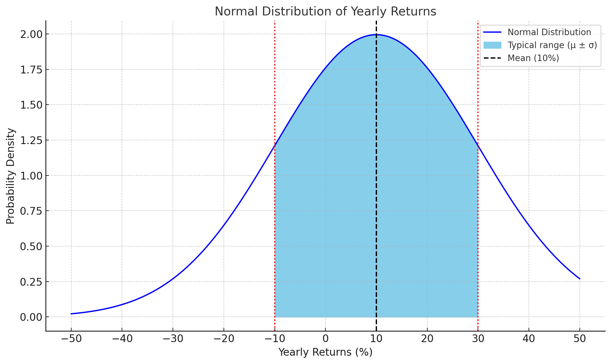
When you invest, your returns won’t be the same every year. Some years you’ll earn a lot, others you might lose money. To make sense of all these ups and downs, we use a concept called standard deviation — it helps describe how much your yearly results tend to move around the average. That average is also called the mean — it’s simply the typical return you’d expect over time. For example, if an investment has a mean (average) return of 10% per year and a standard deviation of 20%, that means in a typical year, your return might fall somewhere between –10% and +30%. That’s because 10% ± 20% covers that range. Statistically, about two-thirds of all outcomes land within that range. Sometimes, of course, the return will be much higher or much lower — those cases are less frequent, but they still happen. This is where the 68–95–99.7 rule comes in: around 68% of yearly results fall within one standard deviation of the mean, 95% within two, and nearly all within three. So if your average return is 10% and the standard deviation is 20%, there’s about a one-in-three chance of losing money in any given year. A bad year like –30% might show up once every six years, while an extreme drop like –50% could happen once in a few decades.
Real investment results don’t always follow this exact bell curve, but the idea still helps us build realistic expectations. Even when the average return looks great, the road there can be bumpy — and knowing that ahead of time can help you stay calm and confident as an investor.
A Quick Example: Calculating Risk Step-by-Step
You don’t need advanced math to grasp how standard deviation is calculated – a simple example can illustrate the concept:
Suppose we have an investment with two equally likely outcomes each year: +30% gain or –10% loss. We want to calculate the expected return and risk (standard deviation) of this investment.
Expected Return (Average):
We already calculated this: (+30% + –10%) / 2 = +10%.
That means we expect to earn an average return of 10% per year. This is called the arithmetic mean.Deviation from the Mean:
Now we check how far each outcome is from that 10% average.
– If we get +30%, that’s 20 percentage points above the average.
– If we get –10%, that’s 20 percentage points below the average.
So the deviations are +20% and –20%.Variance:
We take each deviation (+20% and –20%) and square them (multiply them by themselves). This makes all values positive and gives more weight to larger deviations.
(+20%)² = 400
(–20%)² = 400
Now we take the average of those squared numbers:
(400 + 400) / 2 = 400
This number, 400, is the variance — it measures how spread out the outcomes are from the average.Standard Deviation:
To turn the variance back into a useful percentage, we take the square root of 400:
√400 = 20%
So the standard deviation is 20%. This tells us how much the returns usually move up or down from the average year to year.
What does this result mean? It means the typical variation around the mean is about 20 percentage points. Recall our mean was 10%. So a “typical year” might be +10% ± 20% – which indeed would range from –10% to +30%. That matches exactly our two possible outcomes in this simple scenario! In essence, we found that this investment has an expected return of 10% with a volatility of 20%. If this were a real investment, we’d describe it as “expected return ~10%, standard deviation ~20% per year.”
Interpreting the Risk: An SD of 20% is considered quite volatile. It suggests that in about 2 out of 3 years, returns will be within 20% of the 10% average (i.e. between a 10% loss and a 30% gain). It also implies there is a substantial chance of a negative year. Larger swings are possible too – e.g. a 40% loss would be a 2.5-sigma event in this model, not very common but not impossible.
In practical terms, knowing the standard deviation helps you answer questions like: “How bad could it get in a typical bad year?” or “What’s the range of outcomes I should be mentally prepared for most of the time?” It quantifies volatility risk.
Beyond Volatility: Downside Risk and Semivariance
So far, we talked about risk as if “upside” and “downside” are symmetric – that’s what standard deviation does. But as an investor, you might say: “I don’t mind upside surprises at all – it’s the downside that worries me!” Indeed, many people define risk as “the risk of losing money” or “the chance of falling below a certain target.” This is where downside risk measures come in.
One such measure is called semivariance (and its square root, semi-deviation). Semivariance focuses only on the bad part: it calculates the variance (spread) of returns only for outcomes that are below the average (or below some target threshold). In plainer terms, semivariance asks: How volatile are the downside moves? If an investment sometimes shoots to +50% or +100% (huge upside volatility) but never falls below 0%, the standard deviation might be high (because it swings a lot), but the downside risk is actually low (you never lose money!). Semivariance would correctly reflect that by only considering the zero-and-below deviations.
For example, imagine an asset that in bad cases loses 5%, and in good cases gains 20%. It might have a moderate standard deviation, but its downside semi-deviation is fairly small (only 5% deviations on the downside). Conversely, another asset might frequently have –20% bad years and +20% good years; they might have similar 20% SD, but the second asset clearly has more serious downside potential.
Why consider downside risk? Because many investors care more about the probability and extent of losses than variability per SE. Two investments could have the same standard deviation, say 15%, but for one of them most volatility comes from upside swings, while the other has more downside swings. Standard deviation alone wouldn’t distinguish them, but a downside risk measure would.
That said, it turns out that standard deviation and semivariance often paint a similar picture. If an asset’s returns are roughly symmetric or if upside and downside volatility tend to grow together, then focusing only on downside might not drastically change the risk assessment. Standard deviation also can sometimes give early warnings even before losses occur – for instance, if an investment is swinging wildly (high SD) but hasn’t crashed yet, a high SD alerts you to danger, whereas semivariance might look benign until a crash actually happens.
Nonetheless, it’s good to understand downside risk measures conceptually:
Probability of Loss: One simple downside metric is just “How likely is it that I have a negative return in a given period?” . This probability can often be estimated if you know the mean and SD (assuming a distribution), or from historical frequency.
Value at Risk (VaR): This is a metric that asks: “How bad could it get in a worst-case scenario?” For instance, a 95% VaR might be something like, “There is a 95% chance that in any given year we won’t lose more than X%. (And 5% chance we lose more than X.)” If someone says “1-year 95% VaR is 20%,” it means only 1 in 20 years would we expect to lose more than 20%. VaR focuses squarely on the downside tail.
Shortfall or Target Risk: This measures the risk of failing to meet a specific target.
Downside Beta: In portfolio context, we even look at downside correlation (how an investment co-moves with the market during downturns). This gets technical, but it’s another angle: some assets might only be risky when the overall market is down (which is the worst time), and that is captured by downside beta.
To keep things simple: Semivariance or downside risk measures concentrate on what investors fear – losing money or underperforming expectations. They exclude the happy upside deviations. For practical use, you don’t usually calculate semivariance by hand. But you should conceptually ask: “What’s my chance of a bad outcome here, and how bad might it be?” When comparing investments it can be helpful to compare their downside profiles. For instance, two Stocks might both have an 8% average return, but if Stock A had only one losing year of –5% in a decade while Fund B had three losing years including one –20% crash, Fund A clearly had lower downside risk.
Modern portfolio tools will include some downside risk metrics. These give a fuller picture beyond the standard deviation alone. As an educated investor, it’s good to be aware of them: volatility (SD) tells you about typical fluctuations, while downside risk tells you about the painful moments. Both matter.
Why Understanding Risk Is Crucial (Before You Invest)
You might be thinking, “Alright, I have a handle on returns and risk measures now. But why does this really matter to me as an investor?” The short answer: because knowing the risk upfront helps you make better decisions and sleep easier at night.
Here are a few reasons why understanding risk is so important:
Setting Realistic Expectations: If you know an investment has, say, a 20% standard deviation, you won’t be shocked when your portfolio is down 15% in a rough year – it’s within the expected range. You’ll also know that a year with +30% might be unusually good but possible. This keeps you from panicking at normal volatility or getting carried away by exceptional returns. Many new investors get lured into stocks during a booming bull market (when recent returns look amazing) and don’t appreciate the risks involved. When a inevitable downturn comes and they suffer losses, they panic and sell at the worst time. By understanding risk, you can avoid being blindsided and make a plan you can stick with.
Matching Investments to Your Risk Tolerance: Everyone has a different comfort level with risk. Some people can emotionally and financially handle wild swings; others lose sleep over a 5% dip. By knowing the risk profile (volatility, loss probabilities) of an investment, you can choose those that fit you. For example, if you absolutely cannot afford a big loss due to your life situation or principles, you might stick to low-volatility investments (knowing you’ll get lower returns accordingly). On the other hand, if you’re young, financially secure, and aiming for long-term growth, you might be willing to take on higher risk assets.
Avoiding Fraud and Unrealistic Promises: As mentioned, a clear grasp of risk-return trade-off is your defense against charlatans. If someone promises “high guaranteed returns with no risk,” your internal alarm should ring. Any legitimate investment will outline the risks involved. By reading those and understanding terms like standard deviation, VaR, etc., you can quickly tell if a product is too good to be true. Being knowledgeable about risk metrics makes you a savvy investor who can’t be easily fooled.
Long-Term Success: There’s a saying: “Investing is a marathon, not a sprint.” Risk management is key to surviving the marathon. If you take a gamble that’s too risky (beyond what you understood or can handle), you might face a loss that knocks you out of the game permanently (for example, a 50% loss requires a 100% gain to recover – not trivial). By understanding and respecting risk, you’re more likely to build a sustainable investment strategy. This might involve diversifying – spreading investments so you’re not overly exposed to any single risk.
In summary, understanding investment risk is not about eliminating risk (which is impossible if you want any return) – it’s about knowing what you’re getting into. It empowers you to make informed choices, to prepare mentally and financially for downturns, and to stick to a plan calmly. It also ensures you invest in a manner consistent with your risk tolerance, which ultimately leads to better outcomes and peace of mind.
Conclusion: Knowledge Reduces Fear (But Remember, No Crystal Ball)
Assessing financial risk might sound technical, but as we’ve seen, the core ideas can be understood in plain language. We learned that average returns are not the whole story – the variability of returns (risk) determines what you actually experience over time. We broke down how to measure that variability with standard deviation to get a handle on typical ups-and-downs, and we discussed looking at downside risk to focus on the possibility of losses (because, ultimately, losing money is what investors worry about most). We even did a step-by-step calculation on a simple example to see risk math in action. Most importantly, we highlighted why all this matters: knowing the risk helps you align investments with your comfort and values, and avoid nasty surprises.
Understanding risk doesn’t mean you can predict or prevent all losses – it means you’re aware of them and prepared. As the saying goes, “Plans are useless, but planning is indispensable.” By planning for risk – knowing that a 20% drop can happen and building that into your strategy – you won’t be paralyzed by fear or caught off guard. Instead, you’ll take it in stride and make rational decisions.
In investing, knowledge truly is power. When you comprehend concepts like annualized vs average returns, standard deviation, and downside probability, you transform risk from a scary unknown into a manageable factor. Rather than seeing risk as purely a danger, you’ll recognize it as the price we pay for potential reward. And when managed prudently, risk can be compatible with your financial goals.
To sum up: risk is an inherent part of investing, but it doesn’t have to be a deal-breaker. With clear understanding and careful planning, you can approach investments with confidence and realism.
Portfolio (November 9, 2025)
Overview
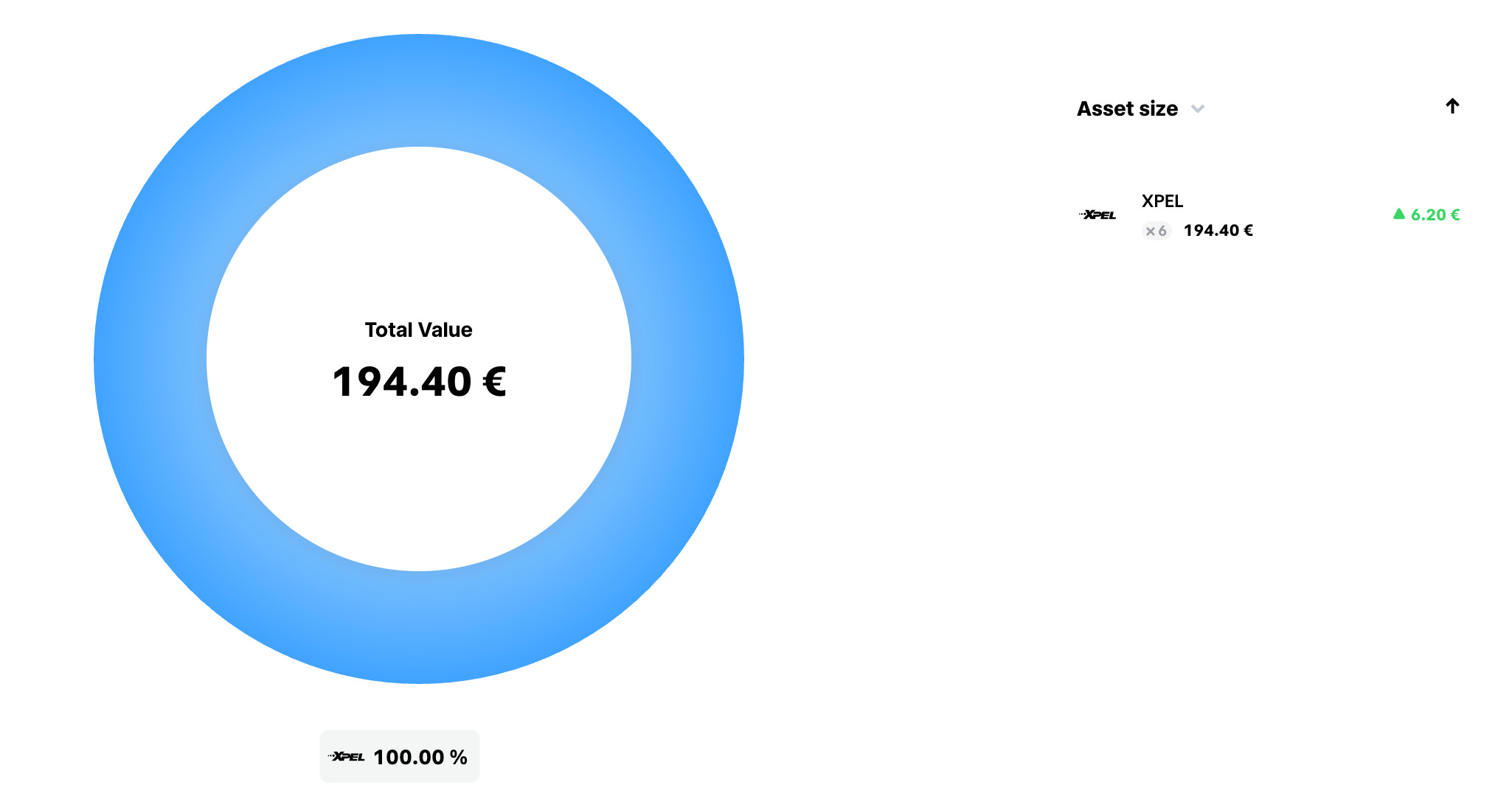
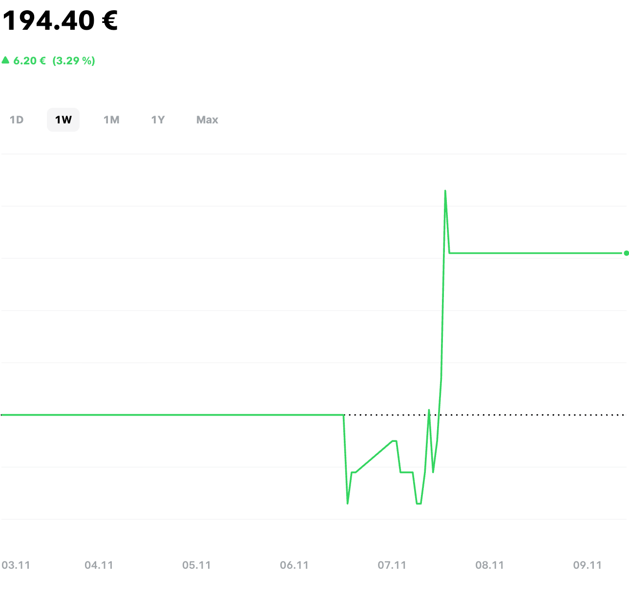
Total Portfolio Value: 206.20 €
Cash: 11.80 €
Stocks: 194.40 €
Positions
XPEL (Ticker: XPEL)
Change: +3.29%
Shares: 6
Entry Price: 31.20 €
Current Value: 194.40 €
Summary: XPEL, Inc. provides protective films and coatings for vehicles, buildings, and other surfaces. Their main products include paint protection films, window films, and ceramic coatings. The company also offers installation services and software for film design.
Deposited Money
Total Deposited: 200 €
Monthly Savings Rate: 200 €
Fees & Taxes
Deposit Fees: 2 €
Order Execution Fees: 1 €
Taxes: 0 €
Stock analysis
XPEL Inc.
Introduction: XPEL Inc. is a U.S.-based company specializing in automotive protective films and coatings.
Core Business
XPEL’s core business is providing protective coverings for vehicles and other surfaces. It produces and distributes paint protection films, window tint films, and ceramic coatings that shield cars (and even architectural or marine assets) from scratches, environmental damage, and wear.
Product Offerings
XPEL offers a range of premium products designed to protect and enhance the longevity of physical assets, especially automobiles:
Paint Protection Film (PPF): A clear urethane film applied to a vehicle’s paint to guard against scratches, stone chips, and UV damage.
Window Tint Films: Tinted films for automotive (and architectural) glass that provide privacy, reduce glare, and block harmful UV rays to protect interiors.
Ceramic Coatings: Liquid coatings (often applied on top of paint) that chemically bond to surfaces, creating a long-lasting protective layer for added shine and easier maintenance.
Competitive Strengths and Innovation
XPEL’s competitive advantages are rooted in quality, innovation, and reach. The company has built a strong reputation for high-quality products that earn customer trust, and it boasts a broad portfolio of protective solutions to meet diverse customer needs. XPEL also invests heavily in research and development to improve its offerings – focusing on product durability, ease of application, and even environmental sustainability – which has led to advanced technologies that often outperform competitors. Another key strength is XPEL’s extensive global distribution and installer network: a robust system of authorized dealers and trained installers, supported by proprietary software tools and ongoing technical training, ensures the company’s products are widely available and consistently applied with high quality. These strengths (brand quality, continuous innovation, and a well-developed delivery network) have solidified XPEL’s position as a leader in its niche of the automotive aftermarket.
Growth Drivers
XPEL’s growth is driven by genuine market demand and strategic, asset-focused expansion – not by speculation. A key tailwind for the business is the increasing number of consumers investing in vehicle protection and customization, which expands the automotive aftermarket and creates real demand for XPEL’s products. In response, the company has been expanding into new high-growth markets through careful partnerships and acquisitions. For example, XPEL acquired its exclusive distributors in major regions like China and India, converting those into direct operations to strengthen its international footprint. Establishing a direct presence in such markets allows XPEL to reinforce its local installer network, enhance customer support and training, and introduce products more efficiently to meet regional needs. This strategy of organic expansion (combined with select strategic acquisitions) means XPEL’s growth is backed by real sales into new territories and deeper market penetration, rather than speculative ventures. Additionally, the company continues to innovate with an eye on sustainability – exploring environmentally friendly product enhancements and improving manufacturing efficiency – to ensure future growth remains grounded in delivering tangible value to customers. Overall, XPEL’s expansion strategy is characterized by responding to actual consumer and industry needs, forging partnerships (such as with car dealerships and OEMs) that integrate its products into the car purchase and maintenance process, and maintaining a long-term focus on quality and sustainability.
Key Business Risks
Like any company in its industry, XPEL faces several business risks arising from market and operational factors.
Key risk factors include:
Competition: The automotive protective film market is crowded with both large, established firms (for example, 3M and Eastman’s Llumar brand) and emerging players, which can lead to pricing pressure and require continuous innovation for XPEL to maintain its market share.
Economic Cycles: XPEL’s performance is tied to trends in the automotive industry; an economic downturn or a decline in vehicle sales could reduce consumer spending on car protection accessories, directly impacting the company’s sales.
Supply Chain & Trade: Disruptions in the supply chain (such as shortages of raw materials or logistics delays) or adverse trade developments (for instance, new tariffs or export/import restrictions) could increase costs or hamper XPEL’s ability to deliver products in certain markets.
Technological Changes: Rapid advances in materials or paint technologies, or competitors introducing superior products, could diminish the need for aftermarket films or erode XPEL’s competitive edge if the company fails to keep pace. XPEL mitigates this by continually investing in R&D, but technological shifts remain an external risk factor.
Conclusion: In summary, XPEL Inc. operates a business centered on automotive protection products. The company’s strengths in innovation and quality. While external challenges such as competition, economic fluctuations, and operational risks exist, XPEL’s focus on real customer demand position it to pursue growth in a responsible manner.

Preview: Next Week
Next week will bring several key U.S. economic data releases that could offer insight into inflation trends and consumer activity — both important factors for understanding the broader market environment.
Upcoming Data Highlights:
Thursday, Nov 13:
Core CPI (m/m) – Previous: 0.2%, Forecast: 0.3%
CPI (m/m) – Previous: 0.3%, Forecast: 0.2%
CPI (y/y) – Current annual inflation rate at 3.0%
Unemployment Claims – Labor market data to watch for potential shifts in employment stability
Friday, Nov 14:
Core PPI (m/m) – Producer inflation indicator
PPI (m/m) – Broader producer price trend
Core Retail Sales (m/m) and Retail Sales (m/m) – Measures of consumer spending momentum
These figures will provide additional context for how inflation and demand are evolving in the U.S. economy — information that remains relevant given the portfolio’s partial exposure to American markets.
In next week’s Deep Dive, we’ll explore more about asset allocation and take a closer look at an interesting company.
Disclaimer: This Post is for informational purposes only and does not constitute financial or investment advice. See the full disclaimer on the Project Compound About page.